Iterative Pruning Methods for Artificial Neural Networks in Julia

A brief survey about compression techniques based on pruning

In recent years, deep learning models have become more popular within real-time embedded applications. In particular, these models have become fundamental in several fields ranging from natural language processing to computer vision. The increases of computational power have been advantageous to face practical challenges that have been resolved by adopting extensive neural networks; as the network grows more in-depth, the model size also increases, introducing redundant parameters which do not contribute towards the specified output. Recently, researchers have focused on different methods on how to reduce storage and computational power by pruning excess parameters without compromising performance.

The reference implementation language for this article is Julia [1], a recently developed programming language oriented towards scientific computing. In particular, we are going to extend the Flux library [2, 3], commonly used in machine learning.

Why pruning?

Pruning algorithms, used since the late \u201980s [4,5], consist in deleting individual weights or entire neurons from the network to reduce redundancy without sacrificing accuracy. In order to obtain good generalization in systems trained by examples, one should use the smallest system that will fit the data [6]. Empirical evidence suggests that it is easier to train a large network and then compress it than to train a smaller network from scratch [7].

The problem with this method is that by removing too many edges one can lose what was learned. The main difficulty is in finding the best model size. Hence, we can see pruning as a neural network architecture search [8] problem, with the goal of finding the optimal network for the considered task. The various implementations of pruning methods differ primarily with respect to four elements:

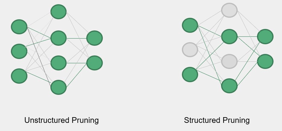
Structure: structured pruning involves the elimination of entire neurons in the network and allows the use of smaller matrices to speed up the computation. Unstructured pruning on the other hand is more flexible because it allows the elimination of single connections, but can not effectively speed up the computation of a neural network.

Saliency: can be seen as the importance associated with each edge, determining whether or not it should be eliminated, depending on the policy adopted
Scheduling: determines the fraction of the network to be eliminated in each step. For example, one-shot pruning consists in eliminating the desired percentage of the network in a single step. Other possible policies are either to eliminate a constant fraction of the network at each step or to adopt a more complex function of scheduling.
Fine-tuning: after the pruning phase, commonly there is a drop in the accuracy, so it might be useful to retrain the network in order to stabilize it. There are different possible approaches to deal with fine-tuning. After the edges elimination one can either train using the same weights that had right before the pruning step (that have not been eliminated), or use a weighing of the edges that had in some previous phase or reinitialize the remaining edges from the beginning

Magnitude Pruning

This is the simplest pruning algorithm. After the common training phase, the connections with lower saliencies are removed. The saliency of a link is only given by the absolute value of its weight. There are two main variants of magnitude pruning. Once a desired percentage of the connections is fixed, the layerwise magnitude pruning will remove that percentage of edges from each layer, while global magnitude pruning will remove a percentage from the entire network without differentiating between layers. More sophisticated techniques of layerwise pruning introduce a sensitivity analysis phase, allowing also to specify different sparsity thresholds for each layer, in order to eliminate more edges in layers that are less sensitive (i.e. those whose elimination of weights affects less the outcome of network). At first, a training phase is always required in order to learn which are the most important connections of the network, those with the highest absolute value. After the elimination of the connections with less saliency,there will be a degrade in the network performance.

For this reason, it is essential to retrain the network starting from the last obtained weights without reinitializing the parameters from scratch. The higher the percentage of pruned parameters the higher the drop in accuracy, this is the reason pruning is usually done iteratively eliminating a small percentage of the network at a time. This implies the need for a schedule, in which we specify the portion of the network we want to delete, in how many steps, and how many connections to eliminate at each step.

Boring preprocessing steps

using Flux: onehotbatch , onecold
using MLDatasets

train_x , train_y = CIFAR10.traindata()
test_x , test_y = CIFAR10.testdata()

X = Flux.flatten(train_x)
Y = onehotbatch(train_y , 0:9)

test_X = Flux.flatten(test_x)
test_Y = onehotbatch(test_y , 0:9)

data = Flux.Data.DataLoader ((X,Y),batchsize = 128, shuffle=true)
test_data = Flux.Data.DataLoader ((test_X ,test_Y), batchsize = 128)

A quick implementation

Pruning is commonly achieved by setting weights to zero and freezing them during subsequent training. My implementation uses an element-wise operation, multiplying the weight matrix by a binary pruning mask.

The first matrix represents the weights of a neural network layer while the second one is themask that sets to zero all the values under a certain threshold, 0.5 in this case

In Flux a simple dense layer is defined by two fundamental parts. First of all, a struct that contains three fields: weight, bias and activation function.

struct Dense{F, M <: AbstractMatrix , B}  
  weight :: M  
  bias::B  
  sigma::F
end

The second key part is the function that expresses the forward step computation as follows:

function(a::Dense)(x:: AbstractVecOrMat)
  W, b, sigma = a.weight , a.bias , a.sigma
  return sigma.(W*x .+ b)
end

The implementation I have developed extends the one provided by Flux by adding the Hadamard product with the matrix mask as described before. A layer PrunableDense then is defined as a struct that reuses the Dense layer with the addition of a field for a bit matrix:

struct PrunableDense  
  dense :: Dense  
  mask:: BitMatrix
end

Secondly, we redefined the forward step function to include the Hadamard product for the mask matrix:

function (a:: PrunableDense)(x:: AbstractVecOrMat)
  W, b,sigma , M = a.dense.W, a.dense.b, a.dense.sigma , a.mask  
  return sigma .((W.*M)*x .+ b)
end

Now you can use these prunable dense layers in the way you wish to create and then reduce the size of your neural network!

Bibliography

[1] Jeff Bezanson, Alan Edelman, Stefan Karpinski, and Viral B Shah. Julia: A fresh approach to numerical computing.SIAM review, 59(1):65\u201398, 2017.

[2] Michael Innes, Elliot Saba, Keno Fischer, Dhairya Gandhi, Marco ConcettoRudilosso, Neethu Mariya Joy, Tejan Karmali, Avik Pal, and Viral Shah. Fashionable modelling with flux.CoRR, abs/1811.01457, 2018.

[3] Mike Innes. Flux: Elegant machine learning with julia.Journal of Open SourceSoftware, 2018.

[4] Steven A. Janowsky. Pruning versus clipping in neural networks.Phys. Rev. A,39:6600\u20136603, Jun 1989

[5] Davis Blalock, Jose Javier Gonzalez Ortiz, Jonathan Frankle, and John Guttag.What is the state of neural network pruning?arXiv preprint arXiv:2003.03033,2020.

[6] Anselm Blumer, Andrzej Ehrenfeucht, David Haussler, and Manfred K Warmuth.Occam\u2019s razor.Information processing letters, 24(6):377\u2013380, 1987.

[7] Russell Reed. Pruning algorithms-a survey.IEEE transactions on Neural Networks, 4(5):740\u2013747, 1993.

[8] Zhuang Liu, Mingjie Sun, Tinghui Zhou, Gao Huang, and Trevor Darrell. Rethinking the value of network pruning, 2019.“}