X-Ray Image Segmentation using U-Nets
FREEIn this article, we shall look at using U-Nets for image segmentation. The link to the blog on Medium is as follows: X-Ray Image Segmentation using U-Nets.
Also, do check out the code for this article! Hope you'll like it.
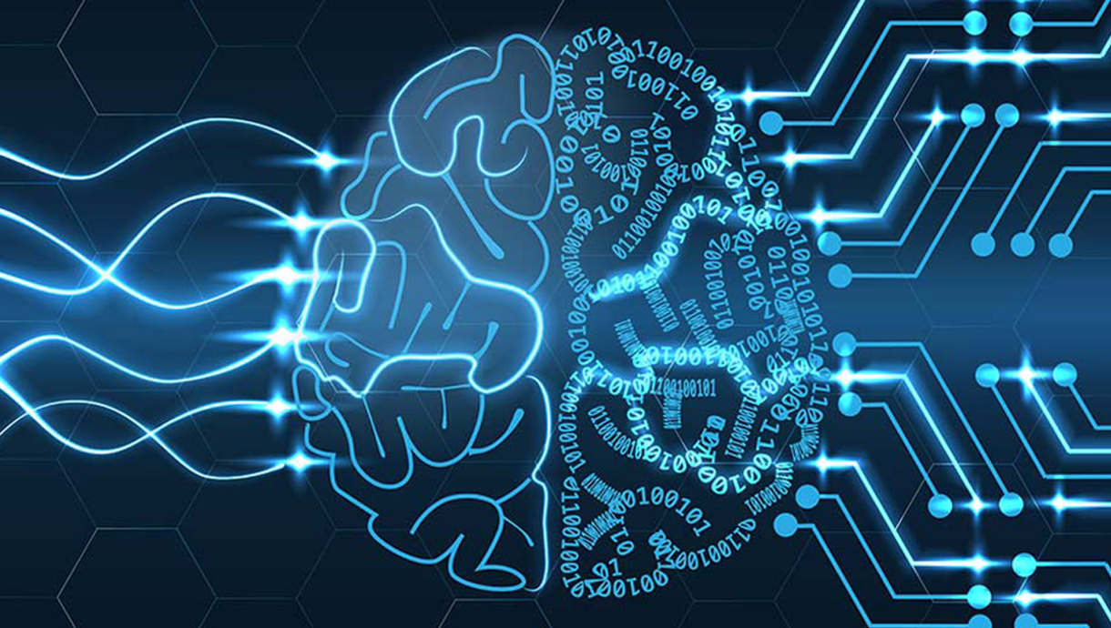
What is Deep Learning?
Deep Learning , as IBM defines it is “an attempt to mimic the human brain albeit far from matching its ability, enabling systems to cluster data and make predictions with incredible accuracy”.
It is essentially a Machine Learning technique that helps teach computers how to learn by example, something which is an innate quality possessed by humans.
| Image credits: L3 Harris |
|---|
 |
What is Image Segmentation?
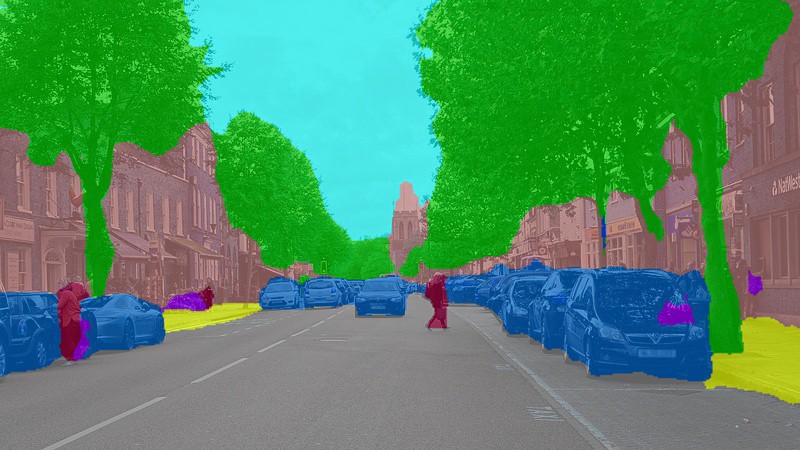
Image segmentation is the process by which an image is broken down into various subgroups called segments. This essentially helps in reducing the complexity of the image to make further processing or analysis of the image much simpler. Image segmentation is generally used to locate objects and boundaries in images.
There are a variety of applications of Image segmentation in various domains. Some of which include: Medical Imaging, Object Detection, Face Recognition, etc.
| Image credits: link |
|---|
 |
What is a U-Net?
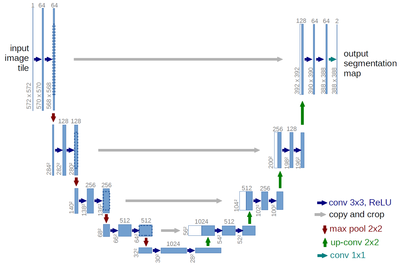
The U-Net is a convolutional network architecture for fast and precise segmentation of biomedical images. Let’s go ahead and discuss the architecture of the U-Net which has been described in the following paper.
In the U-Net, like every other Convolutional Neural Network, it consists of operations such as Convolution and Max Pooling.
Here, as the input image is fed into the network, the data propagates through all the possible paths in the network and at the end, a segmentation map is returned as the output.
In the diagram, each blue box corresponds to a multi-channel feature map. Initially, most of the operations are convolutions followed by a non-linear activation such as ReLU. This is followed by a Max Pooling operations which reduces the size of the feature map. Also, after every Max Pooling operation, the number of feature channels increases by a factor of 2. All in all, the sequence of convolutions and max pooling operations results in a spatial contraction.
The U-Net also has an additional expansion path to create a high-resolution segmentation map. This expansion path consists of a sequence of up-convolutions and concatenation with high-resolution features from contracting path. Followed by this, we get our output segmentation map.
Lung segmentation using a U-Net
For this purpose, I used the Montgomery County X-ray Set . The dataset consists of various x-ray images of lungs along with the images of the segmented images of the left and right lung of each x-ray which have been given separately.
So, after importing the required libraries, the following functions were created to read in the images and masks.
"""To read in the images"""
def imageread(path,width=512,height=512):
    x = cv2.imread(path, cv2.IMREAD_COLOR)
    x = cv2.resize(x, (width, height))
    x = x/255.0
    x = x.astype(np.float32)
    return x

""" To read in the masks"""
def maskread(path_l, path_r,width=512,height=512):
    x_l = cv2.imread(path_l, cv2.IMREAD_GRAYSCALE)
    x_r = cv2.imread(path_r, cv2.IMREAD_GRAYSCALE)
    x = x_l + x_r
    x = cv2.resize(x, (width, height))
    x = x/np.max(x)
    x = x > 0.5
    x = x.astype(np.float32)
    x = np.expand_dims(x, axis=-1)
    return x
Following this, the data was split into train, validation and test sets and was converted into tensors so that it could be fed as an input to the U-Net.
def conv_block(input, num_filters):
    x = Conv2D(num_filters, 3, padding="same")(input)
    x = BatchNormalization()(x)
    x = Activation("relu")(x)

    x = Conv2D(num_filters, 3, padding="same")(x)
    x = BatchNormalization()(x)
    x = Activation("relu")(x)

    return x

def encoder_block(input, num_filters):
    x = conv_block(input, num_filters)
    p = MaxPool2D((2, 2))(x)
    return x, p

def decoder_block(input, skip_features, num_filters):
    x = Conv2DTranspose(num_filters, (2, 2), strides=2, padding="same")(input)
    x = Concatenate()([x, skip_features])
    x = conv_block(x, num_filters)
    return x

def build_unet(input_shape):
    inputs = Input(input_shape)

    s1, p1 = encoder_block(inputs, 64)
    s2, p2 = encoder_block(p1, 128)
    s3, p3 = encoder_block(p2, 256)
    s4, p4 = encoder_block(p3, 512)

    b1 = conv_block(p4, 1024)

    d1 = decoder_block(b1, s4, 512)
    d2 = decoder_block(d1, s3, 256)
    d3 = decoder_block(d2, s2, 128)
    d4 = decoder_block(d3, s1, 64)

    outputs = Conv2D(1, 1, padding="same", activation="sigmoid")(d4)

    model = Model(inputs, outputs, name="U-Net")
    return model
This is the U-Net architecture which was used.
Following this, the following hyperparameters were used for training:
- batch size = 2
- learning rate = 1e-5
- epochs = 30
The model was compiled using the Adam optimizer with the above mentioned learning rate. The metrics used included Dice coefficient, IoU, Recall and Precision.
After training the model over 30 epochs, the model which was saved (with a validation loss of 0.10216) had the following metrics:
- dice_coef: 0.9148
- iou: 0.8441
- recall: 0.9865
- precision: 0.9781
- val_loss: 0.1022
- val_dice_coef: 0.9002
- val_iou: 0.8198
- val_recall: 0.9629
- val_precision: 0.9577
Results
Followed by this, the saved model was used for the purpose of testing. The predictions of the masks on the test set were saved and a combined image of the original image, the original mask and the predicted mask have been given for a few test samples as follows.
| Image credits: Output generated by my code |
|---|
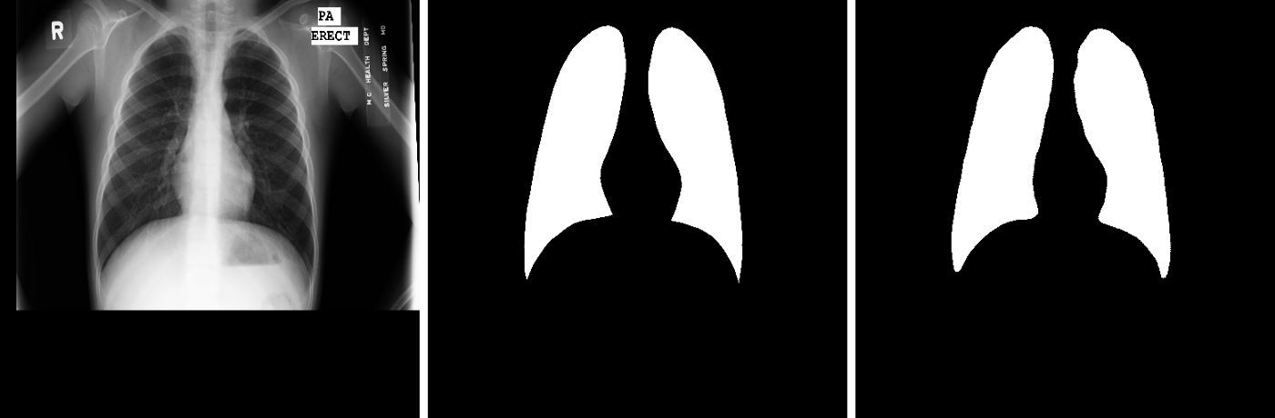 |
| Image credits: Output generated by my code |
|---|
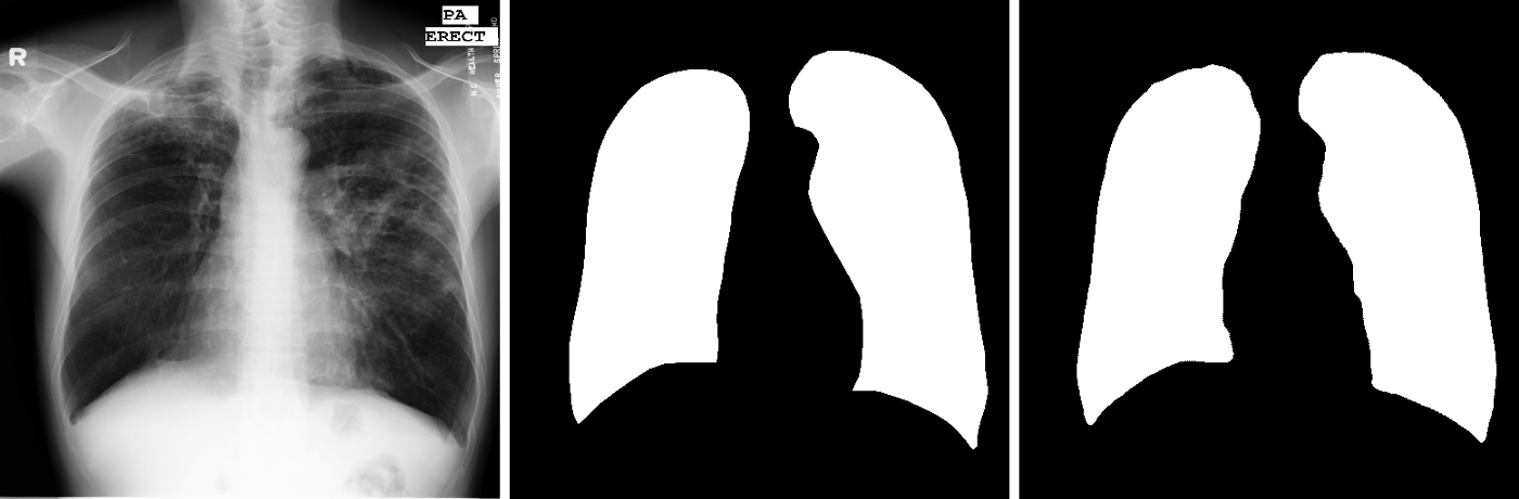 |
The following is the link to the code.
